WARPLab 7
- Downloads
Getting Started
- Sample Buffer Sizes
- Automatic Gain Control
- Examples
- Extending WARPLab
- Debugging Errors
- Porting Code
- Benchmarks
WARPLab 7 Framework
WARPLab 7 Reference Design
Reference Design Modules
- Node
Interface Group
Baseband
Transport
Trigger Manager
Hardware
WARPLab 7 Example: 8x2 Array
File: wl_example_8x2_array.m
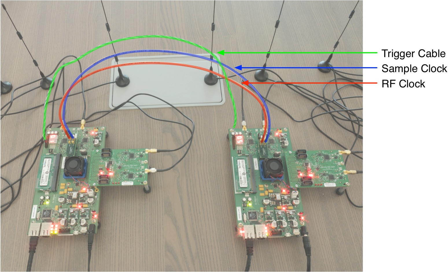
This example shows how WARPLab can be used for array communications even when the number of antennas exceeds what can be supported on a single WARP board. This example uses two separate WARP boards to act as a single many-antenna transmitter while a third board receives their transmissions.
This example uses 3 nodes:
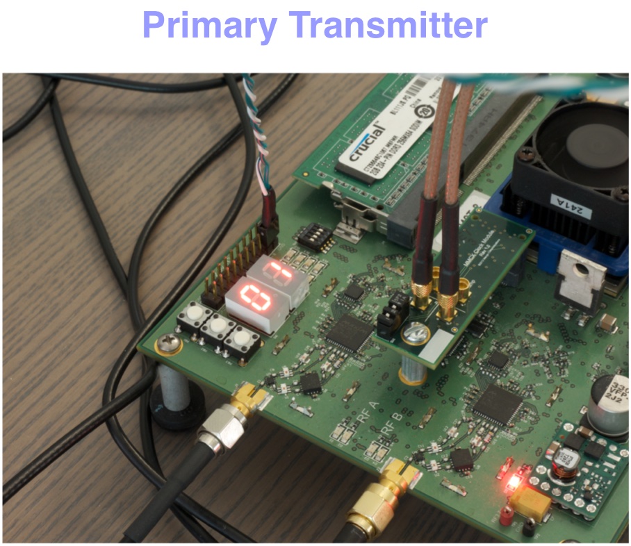
- A node that acts as a primary transmitter. This node uses its own on-board clocks for sampling and RF clocking.
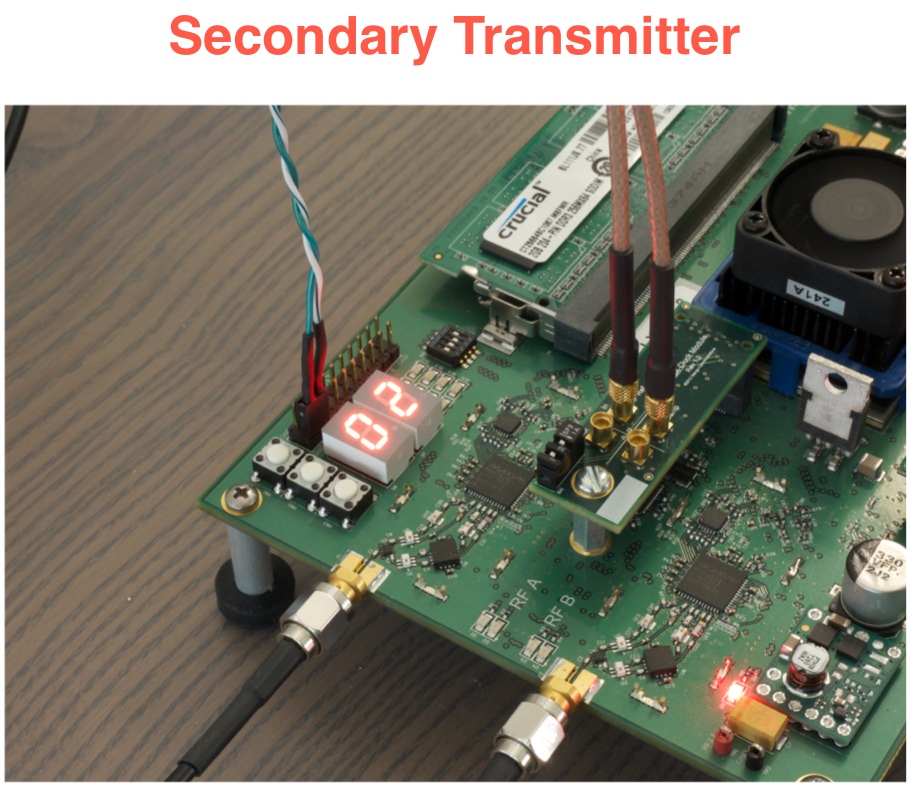
- A node that acts as a secondary transmitter. This node uses the primary transmitter's clocks as the sources for sampling and RF. Furthermore, the Trigger Manager core is used such that the secondary transmitter is triggered by an external twisted pair cable assembly.
- A node to act as a receiver.
Requirements:
- WARPLab reference design 7.1.0 or later
- 2 WARP v3 nodes
- 2 FMC-RF-2X245 radio modules
- Clock connection between WARP boards. Either
- CM-MMCX assembly:
- 2 CM-MMCX clock modules (one per WARP v3 node)
- 2 MMCX cable assemblies
- 1 twisted pair cable assembly
- CM-PLL assembly (requires WARPLab 7.6.0):
- 2 CM-PLL clock modules (one per WARP v3 node)
- 1 CM-PLL compatible cable
- CM-MMCX assembly:
Setup
NOTE: Setup is shown for CM-MMCX modules since that setup is more complicated. If using the CM-PLL module, attach the CM-PLL cable from the OUT header from the primary transmitter to the IN header of the secondary transmitter.

To run this example, you must set up your experiment as follows:
- Mount the CM-MMCX or CM-PLL modules on each WARP v3 node. Power must be off when mounting/unmounting a clock module.
- Mount the FMC-RF-2X245 modules on the same two WARP v3 nodes. For assistance installing an FMC-RF-2X245, see the FMC Installation How-To.
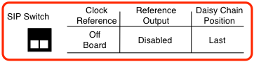
- Set the CM-MMCX or CM-PLL switches on each node (see Clock Configuration settings); one node will be the clock source, the other will be the clock sink.
- Connect clock modules:
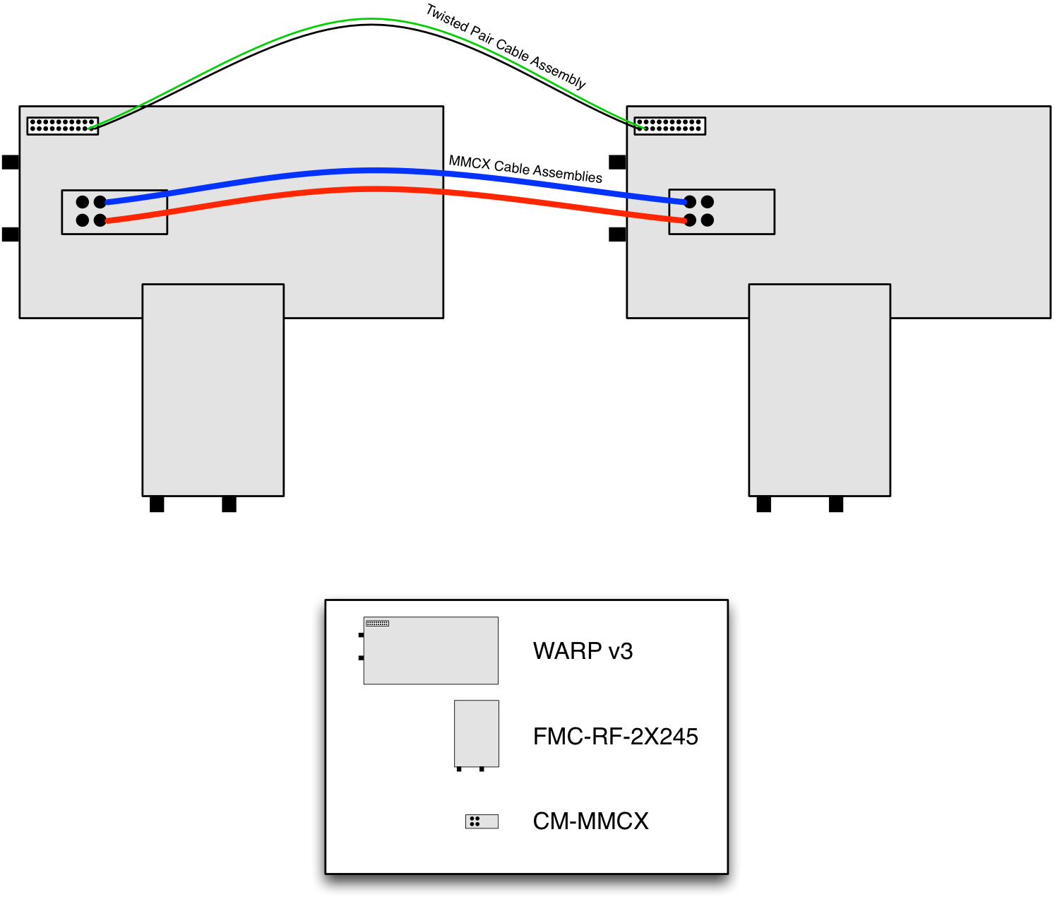
- If using the CM-MMCX modules, connect MMCX cables from the outputs of the source node to the inputs of the sink node. Then, connect the twisted pair cable between the debug headers of the WARP v3 boards. Pin 8 of the source node should connect to pin 15 of the sink node. Use the other conductor of the cable to connect ground between nodes (see figure below).
- If using the CM-PLL modules, connect the cable between the Board-to-board Header OUT of the source node and the Board-to-board Header IN of the sink node.
- Set the DIP switches on the WARP v3 boards to 0000 (clock source node) and 0001 (clock sink node).
- Power on the two WARP v3 nodes
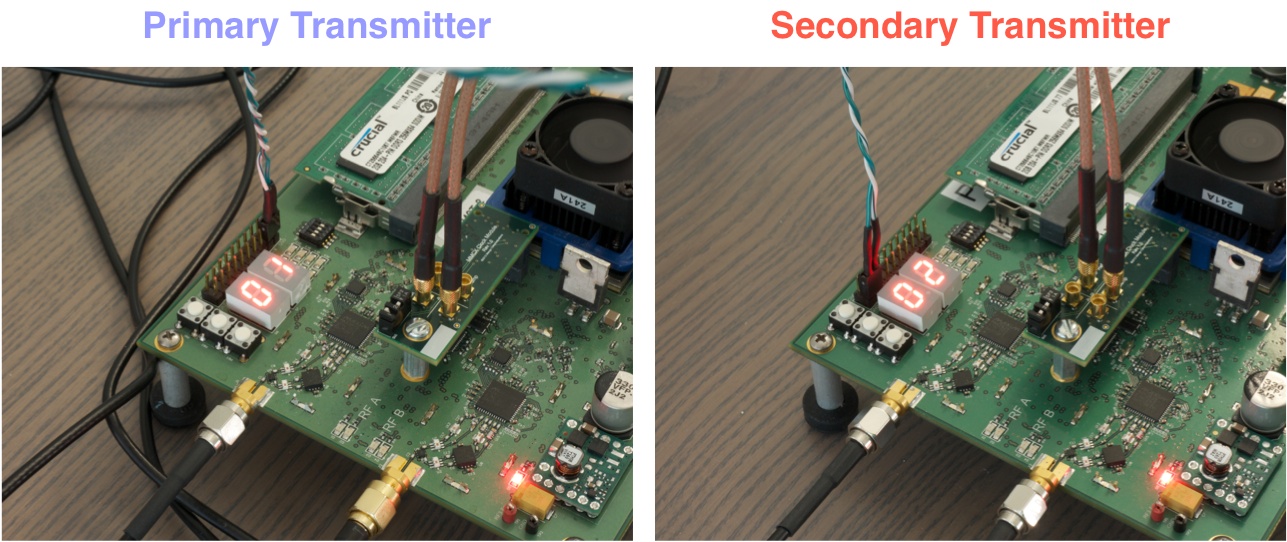
- Download the 4RF WARPLab reference bitstream to both nodes (clock source node first). Both nodes should boot, with the source node showing "01" on the hex displays and the sink showing "02".
- Set the DIP switch on the third WARP v3 board to 0010.
- Power on the third WARP v3 board and download the 2RF WARPLab reference bitstream. The node should boot and show "03" on the hex displays.
Please refer to the WARPLab Hardware Configuration user guide for more details on each of these steps.
 | 
|
| Primary Transmitter Configuration | Secondary Transmitter Configuration |
Photos of Setup
 | 
|
Once the hardware is connected and programmed you can run the example m code: wl_example_8x2_array.m.
Example Overview
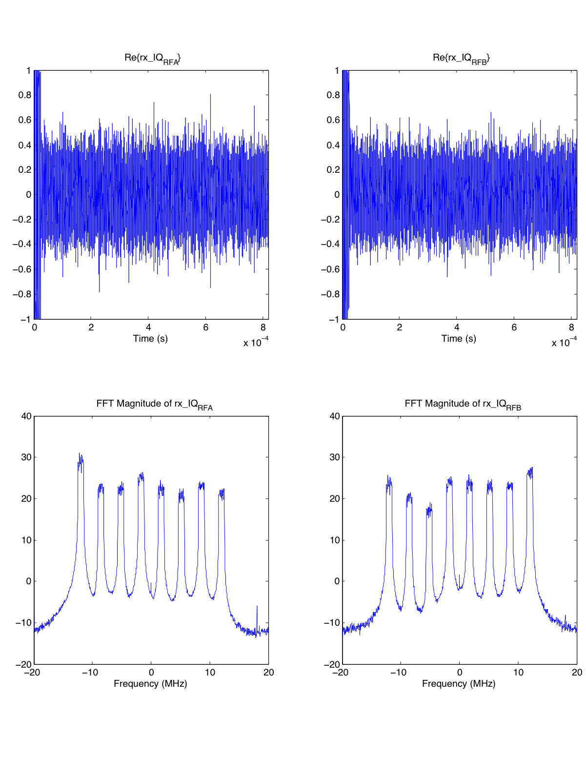
In this example, we use each of the 8 transmit antennas to generate noise that is bandlimited to 1 MHz and digitally mixed to one of 8 different frequencies [-12, -8.5714, -5.1429, -1.7143, 1.7143, 5.1429, 8.5714, 12] MHz. Note: these are frequencies relative to baseband, so 0 MHz corresponds to the center frequency of the radio (Channel 11 of the 2.4 GHz band by default). These 8 different signals are all transmitted simultaneously and are then captured through two receive antennas on the receiving board. Visualizations of those receptions are then plotted.
The purpose of this example is to show how multiple transmit nodes should be synchronized. This technique can scale to arrays even larger than 8 transmit antennas. A similar technique was used in the Rice University Argos Project.
Observations
When you run the example script, it will produce a plot that looks like this

The top-left subplot shows the real part of the received waveform through interface RFA on the board. The top-right subplot shows the real part of the received waveform through interface RFB. The two plots below those show the magnitudes of the signals after FFTs are taken, allowing us to see the 8 different 1 MHz-wide noise signals that were transmitted. Note that the heights (magnitudes) of each of these 8 signals are different due to frequency selective fading. If you change line 15 of wl_example_8x2_array.m to "true," then the script will loop and repeatedly transmit, receive, and produce plots until any key is pressed on the keyboard of the host PC that is running MATLAB. While it is running, you can move antennas around and walk through the room for an interesting animated visualization of frequency selective fading.
Attachments (9)
- 8x2_overview.jpg (313.4 KB) - added by chunter 11 years ago.
- 8x2_cable_macro.jpg (374.8 KB) - added by chunter 11 years ago.
- 8x2_cable_micro.jpg (263.7 KB) - added by chunter 11 years ago.
- 8x2_result.png (208.0 KB) - added by chunter 11 years ago.
- 8x2_diagram.png (110.7 KB) - added by chunter 11 years ago.
- SIP_clock_source.png (9.7 KB) - added by chunter 9 years ago.
- SIP_clock_sink.png (9.8 KB) - added by chunter 9 years ago.
- 8x2_primary.jpg (220.5 KB) - added by chunter 9 years ago.
- 8x2_secondary.jpg (224.5 KB) - added by chunter 9 years ago.
Download all attachments as: .zip